Ocetrac Structure Overview#
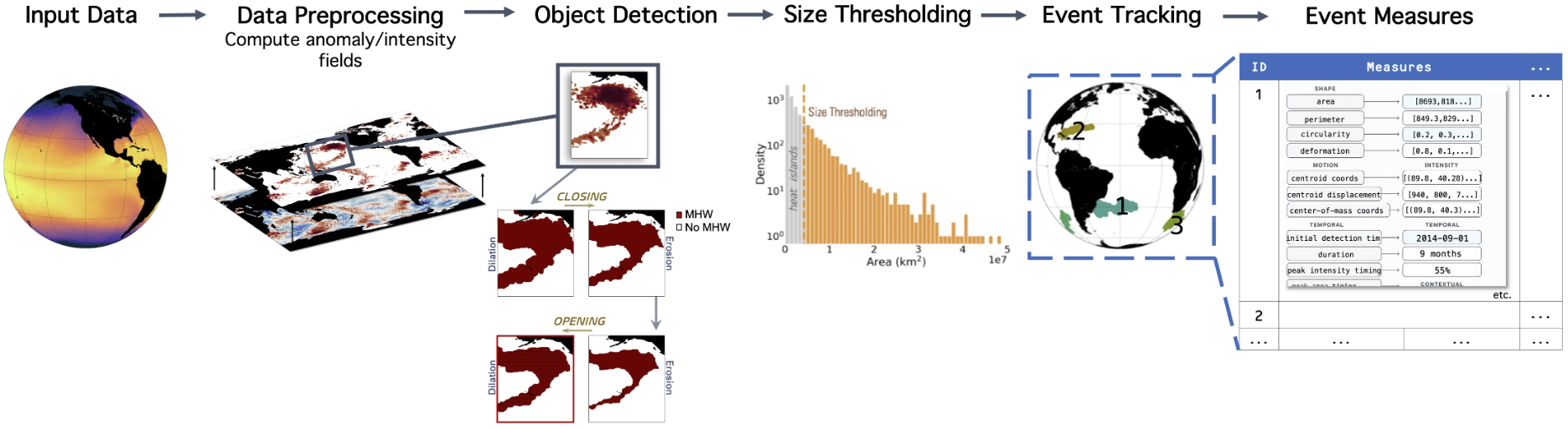
Ocetrac is a tracking framework designed for geophysical feature analysis. While demonstrated here using temperature anomalies to identify marine heatwaves (MHWs), the algorithm is variable-agnostic. It can be applied to any spatiotemporal field that can be thresholded into spatially coherent features and has sufficient temporal resolution to resolve event evolution.
Ocetrac provides two core tracking algorithms, DeepTrack and SurfTrack. Both operate lazily using Dask, enabling efficient processing of large gridded datasets without loading everything into memory at once.

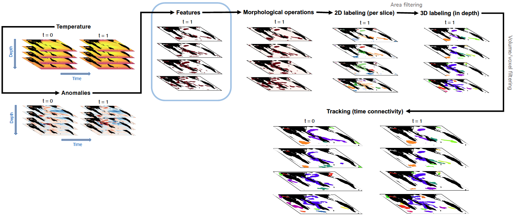
Overview of the six-step Ocetrac processing pipeline for surface (SurfTrack) and subsurface (DeepTrack) feature tracking: (1) input temperature field, (2) anomaly computation, (3) feature detection, (4) morphological operations (closing and opening), (5) area/volume thresholding, and (6) temporal tracking using either permissive (overlap > 0) or restrictive (overlap > user-defined threshold) criteria.#
High-Level Architecture#
DeepTrack operates on four-dimensional fields with dimensions
(time, depth, lat, lon), allowing for the tracking of subsurface features across depth layers
as well as time. SurfTrack operates on one depth layer (such as the surface layer) with
dimensions (time, lat, lon) and is designed for phenomena such as surface marine heatwaves andcold
spells.
Both trackers have a consistent interface: the user provides an xarray.DataArray, a
threshold to define anomalous regions, and a set of morphological parameters controlling how
features are defined and connected. Ocetrac returns a labelled xarray.DataArray where each
integer value corresponds to a unique tracked event.
Input Specifications and Preprocessing#
Both tracking algorithms require input data as an xarray.DataArray. DeepTrack expects dimensions
(time, depth, lat, lon); SurfTrack expects (time, lat, lon). The spatial coordinates
should be latitude and longitude, and the time dimension should be uniformly spaced
to ensure optimal tracking performance. Temporal gaps can be filled using linear interpolation
to maintain continuity.
An optional binary land mask (1 for valid grid cells, 0 for excluded regions such as
land or sea ice) can be provided to omit specific areas from detection and tracking.
All preprocessing, including detrending, anomaly calculation, and thresholding, should be performed before passing data to Ocetrac. Common thresholding approaches include:
Percentile-based — e.g., values exceeding the 90th percentile of anomalies
Absolute value — e.g., values exceeding 28°C
Statistical significance — e.g., values exceeding two standard deviations from the mean
Ocetrac is agnostic to the thresholding method, as long as the input is a binary spatiotemporal field.
DeepTrack Workflow#
The diagram below illustrates the DeepTrack workflow from raw input to labelled output.
run().
Step 1 — Morphological cleaning#
The input field is binarised and morphologically cleaned using a close→open sequence. This produces a
binary DataArray with the same dimensions as the input, where 1 marks anomalous regions and
0 marks background.
Step 2 — 2-D connected-component labelling#
Each (time, depth) slice is labelled independently using 2-D connected-component
labelling. This assigns a unique integer label to each contiguous blob of active cells within
a single depth level and timestep.
Step 3 — Area filtering and depth connectivity#
Small 2-D blobs are removed based on a combined absolute and relative area threshold
(min_area_cells and min_quantile). The surviving blobs are then relabelled and
connected vertically across depth layers using a 3-D structuring element to form
objects. Vertical connectivity can be toggled with the connect_z parameter.
Step 4 — Global volume filter#
3-D objects are ranked globally by voxel count and the smallest fraction (frac_filter)
are discarded. This removes spurious small-scale detections before tracking begins.
Step 5 — Containment-based temporal tracking#
Objects are linked across consecutive timesteps using a containment score that combines
spatial voxel overlap with physical cell volume (when cell_volume is provided). Two
objects are linked if their containment score exceeds contain_thresh. The alpha
parameter controls the weighting between voxel-based and volume-based containment
(0 = volume only, 1 = voxel only). The tracker preserves lineage when objects split
or merge.
Step 6 — Postprocessing#
The tracked array is wrapped as an xarray.DataArray with the same dimensions and
coordinates as the input. Background pixels (event ID = 0) are replaced with NaN.
Implementation example#
import ocetrac

# Initialise DeepTracker with user-defined parameters
tracker = ocetrac.DeepTrack.DeepTracker(
    da,                     # xarray.DataArray (time, depth, lat, lon)
    radius=3,               # morphological disk radius in grid cells
    min_area_cells=200,     # absolute minimum 2-D blob area
    min_quantile=0.25,      # relative area-filter percentile
    contain_thresh=0.3,     # minimum containment score to link objects
    alpha=0.5,              # voxel vs volume containment weight
    frac_filter=0.25,       # drop bottom fraction of 3-D objects
    connect_z=True,         # vertical connectivity in 3-D labelling
    positive=True,          # True for warm anomalies, False for cold
    n_z=20,                 # number of depth levels to use
)

# Run the full pipeline
result = tracker.run(cell_volume=cell_volume_array)

# Or step by step
tracker.clean().label().connect_depth().prefilter().track().postprocess()

# Diagnostics
tracker.summary()
print(tracker.n_events())
print(tracker.event_duration())
SurfTrack Workflow#
SurfTrack operates on three-dimensional data (time, lat, lon) and runs a four-step
pipeline: clean → filter → track → postprocess. Its approach to temporal linking
differs from DeepTrack. Rather than linking objects timestep-by-timestep
using a containment score, SurfTrack applies 3-D connected-component labelling across
the entire (time, lat, lon) cube simultaneously, which produces a looser, more
permissive connectivity in the temporal direction.
The diagram below illustrates the DeepTrack data flow pipeline from raw input to labelled output.
Step 1 — Morphological cleaning (cyclo-symmetric)#
The input field is binarised and a close→open morphological sequence is applied
independently to each (lat, lon) slice using a circular disk structuring element.
Critically, the padding is applied in wrap mode along both spatial axes — this means
the operation is cyclo-symmetric: features near the edges of the domain are treated
as if the grid wraps around periodically, avoiding artefacts at the longitude boundary.
The ocean mask is applied after cleaning to zero out land and sea-ice cells.
- Closing (dilation followed by erosion)
Fills small interior holes and bridges narrow gaps within a feature, maintaining spatial coherence across nearby regions that belong to the same event.
- Opening (erosion followed by dilation)
Removes isolated pixels and residual artefacts introduced by closing, smoothing feature boundaries and eliminating physically spurious detections.
The structuring element radius R controls the spatial scale of filtering. A larger
radius merges nearby features and fills larger gaps; a smaller radius preserves
fine-scale structure at the risk of retaining noise. For 0.25° resolution data:
R= 4–6 grid cells (1–1.5°): Preserves smaller-scale features while removing noiseR= 6–8 grid cells (1.5–2°): Emphasises larger, more coherent structuresR> 8 grid cells: May merge distinct features or fail to identify valid objects
For higher-resolution data, R should be scaled proportionally.
Step 2 — Area filtering#
Each (lat, lon) slice is labelled with 2-D connected components, IDs are made
consecutive across timesteps, and the date-line boundary is handled via
wrap_labels (see below). Objects smaller than the effective area threshold are
then discarded. The effective threshold is defined as the maximum of an absolute minimum area
(min_area_cells) and a relative area threshold based on the distribution of detected
object sizes (the min_size_quartile percentile). This dual thresholding approach ensures
that very small objects are always removed while also adapting to the size distribution of
detected features in the dataset.
Step 3 — 3-D connected-component labelling#
SurfTrack applies 3-D connected-component labelling across the entire
(time, lat, lon) cube simultaneously using connectivity=3 — full 26-connectivity,
meaning face, edge, and corner neighbours are all considered connected in three
dimensions. This is fundamentally different from DeepTrack’s timestep-by-timestep
containment linking: here, any two active voxels that are spatially or temporally
adjacent (including diagonals) within the cube are merged into a single event. This
makes temporal linking looser and more permissive — an object can move diagonally
across both space and time and still be tracked as one continuous event.
For global datasets, wrap_labels is applied after labelling to merge any events
that straddle the 0°/360° longitude boundary into a single consistent event ID.
- Date-line wrapping
The first and last longitude columns are compared after labelling. Any label in the last column that coincides with a label in the first column is reassigned to the first-column label, joining features that cross the date line. Labels are then relabelled to be globally consecutive.
Step 4 — Postprocessing#
The tracked array is wrapped as an xarray.DataArray with the same dimensions and
coordinates as the input. Background pixels are set to NaN. Tracking diagnostics
are stored as DataArray attributes, including initial and final object counts,
the effective area threshold, and the fraction of area accepted and rejected.
Implementation example#
from ocetrac.SurfTrack import SurfTracker

# Initialise SurfTracker with user-defined parameters
tracker = SurfTracker(
    da,                         # xarray.DataArray (time, lat, lon)
    mask,                       # binary ocean mask (lat, lon)
    radius=2,                   # morphological disk radius in grid cells
    min_size_quartile=0.25,     # relative area-filter percentile
    min_area_cells=100,         # absolute minimum object area in grid cells
    timedim='time',             # time dimension name
    xdim='lon',                # longitude dimension name
    ydim='lat',                # latitude dimension name
    positive=True,              # True for warm anomalies, False for cold
)

# Run the full pipeline
result = tracker.run()

# Or step by step
tracker.clean().filter().track().postprocess()

# Diagnostics
tracker.summary()
print(tracker.n_events())
print(tracker.event_duration())
Key Concepts#
- Threshold
The user supplies a scalar threshold that defines what counts as an anomalous region. Grid cells exceeding this threshold are set to
Truein the binary mask; all others are set toFalse.- Morphological parameters
Dilation and erosion operations are applied to the binary mask using a circular structuring element of radius
R. In SurfTrack the padding is applied inwrapmode, making the operation cyclo-symmetric — features near the longitude boundary are treated as if the grid is periodic. A largerRmerges nearby features; a smallerRpreserves finer structure at the risk of retaining noise.- Connectivity (SurfTrack vs DeepTrack)
SurfTrack applies 3-D connected-component labelling with
connectivity=3(full 26-connectivity) across the entire(time, lat, lon)cube simultaneously. This is a loose, permissive approach where any two active voxels that are adjacent in space or time (including diagonals) are part of the same event. DeepTrack instead links objects timestep-by-timestep using a containment score, which is more conservative and explicit about what constitutes a connected event.- Containment score (DeepTrack only)
DeepTrack links objects across timesteps using a containment score that combines voxel overlap with physical cell volume. The
alphaparameter weights these two components (0= volume only,1= voxel only). Objects are linked only if their score exceedscontain_thresh.- Minimum area filter
Small objects are discarded after labelling. In SurfTrack the effective threshold is
max(min_area_cells, percentile(areas, min_size_quartile)). In DeepTrack this is controlled separately at the 2-D level (min_area_cells,min_quantile) and at the 3-D level (frac_filter).- Event ID
Each tracked event is assigned a unique positive integer ID consistent across timesteps. Background pixels are set to
NaNin both trackers. Event IDs can be used to index into the output array and extract the full spatiotemporal footprint of any individual event.- Dask integration
All operations are applied lazily. The tracker builds a computation graph without executing any computation until
.compute()is called or the result is written to disk. This allows Ocetrac to handle datasets that are larger than available memory. Chunking along the time dimension is recommended for optimal performance.