SurfTrack#
SurfTrack operates on 3-D data (time, lat, lon) and uses:
Morphological close→open to clean the binary field
Area filtering to remove small noise objects
3-D connected-component labelling across time and space
Date-line wrapping for global datasets
For subsurface (4-D) tracking see the DeepTrack tutorial.
1. Imports#
[2]:
from ocetrac.SurfTrack import SurfTracker
from ocetrac.preprocessing.cesm2_lens_utils import get_ds_var
from ocetrac.preprocessing.preprocessing import calculate_anomalies_trend_features
[9]:
import numpy as np
import xarray as xr

import cmocean
import cartopy
import cartopy.crs as ccrs
import cartopy.feature as cfeature
from cartopy.mpl.ticker import LongitudeFormatter,LatitudeFormatter
from cartopy.util import add_cyclic_point
import matplotlib.pyplot as plt
import matplotlib.patches as mpatches
from matplotlib.patches import Rectangle
import matplotlib.dates as mdates

import warnings

warnings.filterwarnings("ignore", message=".*decode the variable.*")
warnings.filterwarnings("ignore", message=".*default value for data_vars.*")
2. Data loading#
This section loads CESM2 Large Ensemble (CESM2-LENS) SST data for a single ensemble member. The CESM2-LE provides 100 ensemble members spanning 1850-2100.
Component:
atm(atmosphere model component)Temporal resolution: Monthly means
[16]:
%%time

ens_memb_index = 0
var, comp  = 'SST', 'atm'
directory  = f'/glade/campaign/cgd/cesm/CESM2-LE/{comp}/proc/tseries/month_1/{var}/'

ds_hist, _ = get_ds_var(directory, var, comp, ens_memb_index)

nlat_low, nlat_high = 26, 328
da_sst = ds_hist[var].sel(
    lat=slice(-65, 65),
    time=slice('1979-01', '2015-01')).compute()

print(f"Loaded: {da_sst.dims}  {da_sst.shape}")
Loaded: ('time', 'lat', 'lon')  (433, 138, 288)
CPU times: user 708 ms, sys: 52.4 ms, total: 760 ms
Wall time: 940 ms
[29]:
# Replace 0s with NaN (land masking)
da_sst_noland = da_sst.where(da_sst != 0, np.nan)
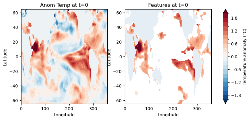
3. Anomaly computation#
This preprocessing step is separate from the Ocetrac tracking algorithm. It prepares the temperature field by the trend and seasonality.
This example notebook uses preprocessing.calculate_anomalies_trend_features, which fits a 6-coefficient harmonic model per grid cell and returns the residual as well as provides the features.
[23]:
%%time

mean, trend, seas, features, anom = calculate_anomalies_trend_features(
    da_sst,
    0.9)

print(f"features shape: {features.shape}  ({features.nbytes/1e9:.2f} GB)")
features shape: (433, 138, 288)  (0.14 GB)
CPU times: user 1.35 s, sys: 72 ms, total: 1.42 s
Wall time: 1.52 s
[24]:
# Subset first 40 timesteps (months) for tutorial
features = features.isel(time=slice(40))
[ ]:
da_sst_noland = da_sst.where(da_sst != 0, np.nan)
[28]:
## -------------- Figure of anom temperature and features

fig, (ax1, ax2) = plt.subplots(1, 2, figsize=(10, 4))

im1 = anom[30, :, :].plot.contourf(
    ax=ax1,
    levels=21,
    vmin=-2,
    vmax=2,
    cmap='RdBu_r',
    add_colorbar=False
)
ax1.set_title('Anom Temp at t=0', fontsize=12)
ax1.set_xlabel('Longitude')
ax1.set_ylabel('Latitude')

im2 = features[30, :, :].plot.contourf(
    ax=ax2,
    levels=21,
    vmin=-2,
    vmax=2,
    cmap='RdBu_r',
    add_colorbar=False
)
ax2.set_title('Features at t=0', fontsize=12)
ax2.set_xlabel('Longitude')
ax2.set_ylabel('Latitude')

cbar = plt.colorbar(im1, ax=[ax1, ax2], orientation='vertical', pad=0.05)
cbar.set_label('Temperature anomaly (°C)', fontsize=10)

plt.show()
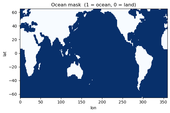
4. Build the ocean mask#
[35]:
mask = xr.where(da_sst[0,:,:] == 0., 0., 1.)

fig, ax = plt.subplots(figsize=(6, 4))
mask.plot(ax=ax, cmap='Blues', add_colorbar=False)
ax.set_title('Ocean mask  (1 = ocean, 0 = land)')
plt.tight_layout(); plt.show(); plt.close()
5. Initialise and run the tracker#
Parameter |
Description |
|---|---|
|
Structuring element radius for morphological close→open. Larger fills wider gaps but risks bridging nearby separate events. |
|
Drop blobs below this percentile of the area distribution. Combined with |
|
Absolute minimum blob size in grid cells. Always applied regardless of the percentile. |
|
|
Morphological cleaning (cyclo-symmetric)#
The input field is binarised and a close→open morphological sequence is applied independently to each (lat, lon) slice using a circular disk structuring element. Critically, the padding is applied in wrap mode along both spatial axes — this means the operation is cyclo-symmetric: features near the edges of the domain are treated as if the grid wraps around periodically, avoiding artefacts at the longitude boundary. The ocean mask is applied after cleaning to zero out land and sea-ice
cells.
Closing (dilation followed by erosion) Fills small interior holes and bridges narrow gaps within a feature, maintaining spatial coherence across nearby regions that belong to the same event.
Opening (erosion followed by dilation) Removes isolated pixels and residual artefacts introduced by closing, smoothing feature boundaries and eliminating physically spurious detections.
The structuring element radius R controls the spatial scale of filtering. A larger radius merges nearby features and fills larger gaps; a smaller radius preserves fine-scale structure at the risk of retaining noise. For 0.25° resolution data:
R= 4–6 grid cells (1–1.5°): Preserves smaller-scale features while removing noiseR= 6–8 grid cells (1.5–2°): Emphasises larger, more coherent structuresR> 8 grid cells: May merge distinct features or fail to identify valid objects
For higher-resolution data, R should be scaled proportionally.
Area filtering#
Each (lat, lon) slice is labelled with 2-D connected components, IDs are made consecutive across timesteps, and the date-line boundary is handled via wrap_labels (see below). Objects smaller than the effective area threshold are then discarded. The effective threshold is defined as the maximum of an absolute minimum area (min_area_cells) and a relative area threshold based on the distribution of detected object sizes (the min_size_quartile percentile). This dual thresholding
approach ensures that very small objects are always removed while also adapting to the size distribution of detected features in the dataset.
[38]:
%%time
tracker = SurfTracker(
    features,
    mask,
    radius            = 2,
    min_size_quartile = 0.25,
    min_area_cells    = 100,
    timedim           = 'time',
    xdim              = 'lon',
    ydim              = 'lat',
    positive          = True,
)
result = tracker.run()
tracker.summary()
Step 1 · morphological cleaning …
    fraction flagged = 0.1022  (OK)
Step 2 · area filtering …
area threshold : 100 cells  (floor=100, percentile=22.0)
Step 3 · 3-D connected-component labelling …
    initial objects : 791
    final objects   : 60
Step 4 · wrapping result …
    final events: 60
=======================================================
SurfTracker — Result Summary
=======================================================
  Input shape    : (40, 138, 288)
  Tracked events : 60
  Duration  min/median/max : 1 / 1 / 22
    >=  1 ts : 60
    >=  3 ts : 20
    >=  6 ts : 11
    >= 12 ts : 5

  Parameters:
    radius               = 2
    min_area_cells       = 100
    min_size_quartile    = 0.25
    positive             = True
=======================================================
CPU times: user 1.01 s, sys: 27.2 ms, total: 1.04 s
Wall time: 1.18 s
6. Attributes#
[39]:
print("Attributes:")
for k, v in result.attrs.items():
    print(f"  {k:<30} {v}")
Attributes:
  initial objects identified     791
  final objects tracked          60
  radius                         2
  size quantile threshold        0.25
  min area cells                 100
  min area (effective)           100.0
  percent area reject            0.10522655374881522
  percent area accept            0.8947734462511848
Run steps separately#
[40]:
tracker2 = SurfTracker(
    features, mask,
    radius=2, min_size_quartile=0.25, min_area_cells=100,
    timedim='time', xdim='lon', ydim='lat',
)

# Step 1 — morphological cleaning + masking
tracker2.clean()
frac = float(tracker2.binary_clean.values.mean())
print(f"Step 1 done — fraction flagged warm: {frac:.4f}")

# Step 2 — area filtering
tracker2.filter()
print(f"Step 2 done — effective area threshold: {tracker2.min_area:.0f} cells")
print(f"             initial objects: {tracker2.N_initial}")

# Step 3 — 3-D connected-component labelling + date-line wrap
tracker2.track()

# Step 4 — package result
tracker2.postprocess()
print(f"Step 4 done — final events: {tracker2.n_events()}")
Step 1 · morphological cleaning …
    fraction flagged = 0.1022  (OK)
Step 1 done — fraction flagged warm: 0.1022
Step 2 · area filtering …
area threshold : 100 cells  (floor=100, percentile=22.0)
Step 2 done — effective area threshold: 100 cells
             initial objects: 791
Step 3 · 3-D connected-component labelling …
    initial objects : 791
    final objects   : 60
Step 4 · wrapping result …
    final events: 60
Step 4 done — final events: 60
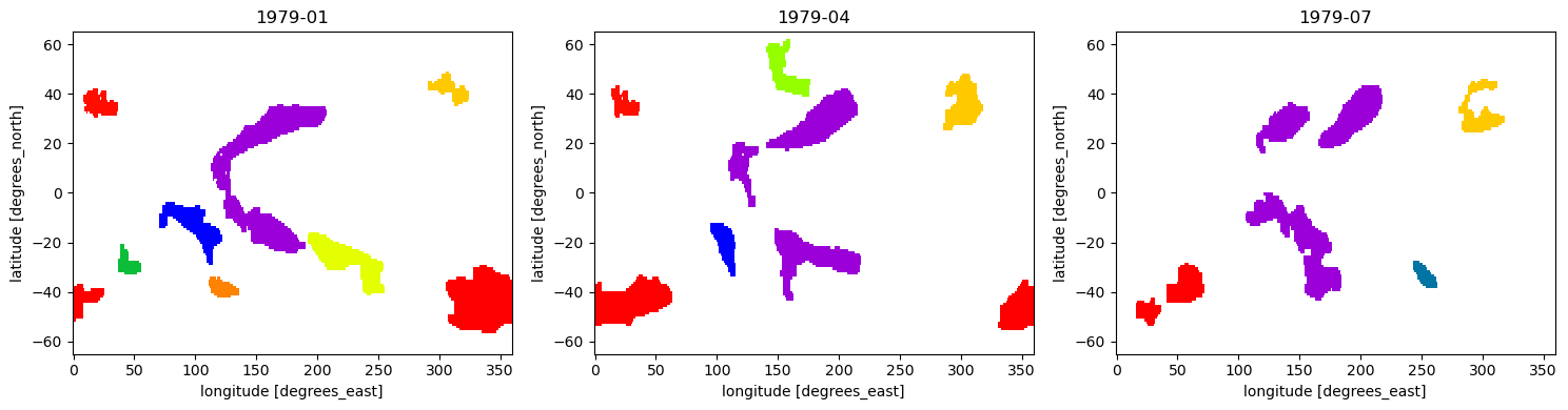
8. Plotting and Inspection#
[41]:
def plot_surface_labels(result, timesteps, cmap='prism'):
    vmax = int(np.nanmax(result.values))
    fig, axes = plt.subplots(1, len(timesteps), figsize=(5 * len(timesteps), 4))
    if len(timesteps) == 1:
        axes = [axes]
    for ax, t in zip(axes, timesteps):
        result.isel(time=t).plot(
            ax=ax, cmap=cmap, vmin=1, vmax=vmax, add_colorbar=False
        )
        try:
            t_label = str(result.time.values[t])[:7]
        except Exception:
            t_label = f't={t}'
        ax.set_title(t_label)
    plt.tight_layout(); plt.show(); plt.close()

plot_surface_labels(result, timesteps=list(range(0, min(9, result.shape[0]), 3)))
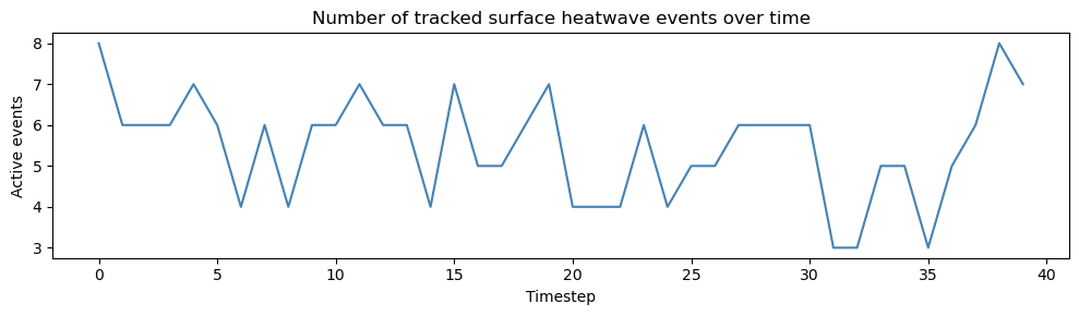
[42]:
n_per_t = [
    len(np.unique(result.isel(time=t).values[
        ~np.isnan(result.isel(time=t).values)
    ]))
    for t in range(result.shape[0])
]

fig, ax = plt.subplots(figsize=(10, 3))
ax.plot(n_per_t, lw=1.5, color='steelblue')
ax.set_xlabel('Timestep'); ax.set_ylabel('Active events')
ax.set_title('Number of tracked surface heatwave events over time')
plt.tight_layout(); plt.show(); plt.close()
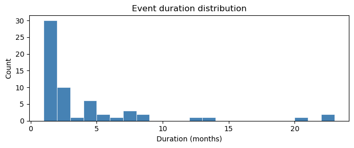
[43]:
durations = tracker.event_duration()
durs      = np.array(list(durations.values()))

print(f"Total events        : {len(durs)}")
print(f"Duration min/median/max : "
      f"{durs.min()} / {int(np.median(durs))} / {durs.max()}")
print(f"  1 ts  : {(durs == 1).sum()}")
print(f"  2 ts  : {(durs == 2).sum()}")
print(f"  >= 3  : {(durs >= 3).sum()}")

fig, ax = plt.subplots(figsize=(7, 3))
ax.hist(durs, bins=range(1, durs.max() + 2), edgecolor='white', linewidth=0.5,
        color='steelblue')
ax.set_xlabel('Duration (months)'); ax.set_ylabel('Count')
ax.set_title('Event duration distribution')
plt.tight_layout(); plt.show(); plt.close()
Total events        : 60
Duration min/median/max : 1 / 1 / 22
  1 ts  : 30
  2 ts  : 10
  >= 3  : 20